pacman::p_load(sf,tmap,sfdep, tidyverse, spdep)In-class Exercise 6: Spatial Weights sfdep methods
1 Importing
INSERT IMG
2 The Data
For the purpose of this in-class exercise, the Hunan data sets will be used.
There are two data sets in this use case, they are:
Hunan, a geospatial data set in ESRI shapefile format, and
Hunan_2012, an attribute data set in csv format.
2.1 Aspatial
hunan2012 <- read_csv("data/aspatial/Hunan_2012.csv")2.2 Geospatial
hunan <- st_read(dsn = "data/geospatial",
                 layer = "Hunan")
Reading layer `Hunan' from data source
`C:\tiffanik\IS415-GAA\In-class_Ex\In-class_Ex06\data\geospatial'
using driver `ESRI Shapefile'
Simple feature collection with 88 features and 7 fields
Geometry type: POLYGON
Dimension: XY
Bounding box: xmin: 108.7831 ymin: 24.6342 xmax: 114.2544 ymax: 30.12812
Geodetic CRS: WGS 842.3 Performing relational join
LEFT = sf df
RIGHT = tpler df
hunan_GDPPC <- left_join(hunan,hunan2012)%>%
  select(1:4, 7, 15)
3 Visualising Regional Development Indicator
tmap_mode("plot")
tm_shape (hunan_GDPPC) +
  tm_fill("GDPPC",
          style = "quantile",
          palette = "Blues",
          title = "GDPPC") +
tm_layout ( main.title = "Distribution of GDP per capita by distribution",
            main.title.position = "left",
            main.title.size = 1.2,
            legend.height = 0.45,
            legend.width = 0.35,
            frame = TRUE) +
tm_borders (alpha = 0.5) +
tm_compass (type="8star", size = 2) +
tm_scale_bar() +
tm_grid(alpha =0.2)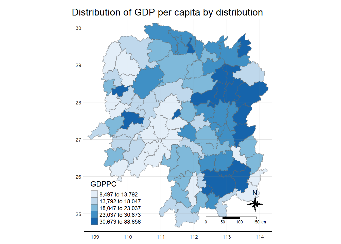
3.1 Contiguity neighbours method
In the code chunk below st_contiguity() is used to derive a contiguity neighbour list by using Queen’s method.
cn_queen <- hunan_GDPPC %>%

mutate(nb = st_contiguity (geometry),

.before = 1)
With the below method then the above is redundant
rook method
c_rook < - hunan_GDPPC %>%
mutate(nb = st_contiguity (geometry),
queen = FALSE,
.before = 1)
wm_q <- hunan_GDPPC %>%
mutate(nb = st_contiguity (geometry),
        wt = st_weights (nb),
.before = 1)
wm_q <- poly2nb(hunan_GDPPC, queen=TRUE)
summary(wm_q)Neighbour list object:
Number of regions: 88
Number of nonzero links: 448
Percentage nonzero weights: 5.785124
Average number of links: 5.090909
Link number distribution:
1 2 3 4 5 6 7 8 9 11
2 2 12 16 24 14 11 4 2 1
2 least connected regions:
30 65 with 1 link
1 most connected region:
85 with 11 linkswm_q[[1]][1] 2 3 4 57 85hunan_GDPPC$County[1][1] "Anxiang"hunan_GDPPC$NAME_3[c(2,3,4,57,85)][1] "Hanshou" "Jinshi" "Li" "Nan" "Taoyuan"nb1 <- wm_q[[1]]
nb1 <- hunan_GDPPC$GDPPC[nb1]
nb1[1] 20981 34592 24473 21311 22879str(wm_q)List of 88
$ : int [1:5] 2 3 4 57 85
$ : int [1:5] 1 57 58 78 85
$ : int [1:4] 1 4 5 85
$ : int [1:4] 1 3 5 6
$ : int [1:4] 3 4 6 85
$ : int [1:5] 4 5 69 75 85
$ : int [1:4] 67 71 74 84
$ : int [1:7] 9 46 47 56 78 80 86
$ : int [1:6] 8 66 68 78 84 86
$ : int [1:8] 16 17 19 20 22 70 72 73
$ : int [1:3] 14 17 72
$ : int [1:5] 13 60 61 63 83
$ : int [1:4] 12 15 60 83
$ : int [1:3] 11 15 17
$ : int [1:4] 13 14 17 83
$ : int [1:5] 10 17 22 72 83
$ : int [1:7] 10 11 14 15 16 72 83
$ : int [1:5] 20 22 23 77 83
$ : int [1:6] 10 20 21 73 74 86
$ : int [1:7] 10 18 19 21 22 23 82
$ : int [1:5] 19 20 35 82 86
$ : int [1:5] 10 16 18 20 83
$ : int [1:7] 18 20 38 41 77 79 82
$ : int [1:5] 25 28 31 32 54
$ : int [1:5] 24 28 31 33 81
$ : int [1:4] 27 33 42 81
$ : int [1:3] 26 29 42
$ : int [1:5] 24 25 33 49 54
$ : int [1:3] 27 37 42
$ : int 33
$ : int [1:8] 24 25 32 36 39 40 56 81
$ : int [1:8] 24 31 50 54 55 56 75 85
$ : int [1:5] 25 26 28 30 81
$ : int [1:3] 36 45 80
$ : int [1:6] 21 41 47 80 82 86
$ : int [1:6] 31 34 40 45 56 80
$ : int [1:4] 29 42 43 44
$ : int [1:4] 23 44 77 79
$ : int [1:5] 31 40 42 43 81
$ : int [1:6] 31 36 39 43 45 79
$ : int [1:6] 23 35 45 79 80 82
$ : int [1:7] 26 27 29 37 39 43 81
$ : int [1:6] 37 39 40 42 44 79
$ : int [1:4] 37 38 43 79
$ : int [1:6] 34 36 40 41 79 80
$ : int [1:3] 8 47 86
$ : int [1:5] 8 35 46 80 86
$ : int [1:5] 50 51 52 53 55
$ : int [1:4] 28 51 52 54
$ : int [1:5] 32 48 52 54 55
$ : int [1:3] 48 49 52
$ : int [1:5] 48 49 50 51 54
$ : int [1:3] 48 55 75
$ : int [1:6] 24 28 32 49 50 52
$ : int [1:5] 32 48 50 53 75
$ : int [1:7] 8 31 32 36 78 80 85
$ : int [1:6] 1 2 58 64 76 85
$ : int [1:5] 2 57 68 76 78
$ : int [1:4] 60 61 87 88
$ : int [1:4] 12 13 59 61
$ : int [1:7] 12 59 60 62 63 77 87
$ : int [1:3] 61 77 87
$ : int [1:4] 12 61 77 83
$ : int [1:2] 57 76
$ : int 76
$ : int [1:5] 9 67 68 76 84
$ : int [1:4] 7 66 76 84
$ : int [1:5] 9 58 66 76 78
$ : int [1:3] 6 75 85
$ : int [1:3] 10 72 73
$ : int [1:3] 7 73 74
$ : int [1:5] 10 11 16 17 70
$ : int [1:5] 10 19 70 71 74
$ : int [1:6] 7 19 71 73 84 86
$ : int [1:6] 6 32 53 55 69 85
$ : int [1:7] 57 58 64 65 66 67 68
$ : int [1:7] 18 23 38 61 62 63 83
$ : int [1:7] 2 8 9 56 58 68 85
$ : int [1:7] 23 38 40 41 43 44 45
$ : int [1:8] 8 34 35 36 41 45 47 56
$ : int [1:6] 25 26 31 33 39 42
$ : int [1:5] 20 21 23 35 41
$ : int [1:9] 12 13 15 16 17 18 22 63 77
$ : int [1:6] 7 9 66 67 74 86
$ : int [1:11] 1 2 3 5 6 32 56 57 69 75 ...
$ : int [1:9] 8 9 19 21 35 46 47 74 84
$ : int [1:4] 59 61 62 88
$ : int [1:2] 59 87
- attr(*, "class")= chr "nb"
- attr(*, "region.id")= chr [1:88] "1" "2" "3" "4" ...
- attr(*, "call")= language poly2nb(pl = hunan_GDPPC, queen = TRUE)
- attr(*, "type")= chr "queen"
- attr(*, "sym")= logi TRUE3.2 Creating (ROOK) contiguity based neighbours
wm_r <- poly2nb(hunan_GDPPC, queen=FALSE)
summary(wm_r)
Neighbour list object:
Number of regions: 88
Number of nonzero links: 440
Percentage nonzero weights: 5.681818
Average number of links: 5
Link number distribution:
1 2 3 4 5 6 7 8 9 10
2 2 12 20 21 14 11 3 2 1
2 least connected regions:
30 65 with 1 link
1 most connected region:
85 with 10 links3.3 Visualising contiguity weights
longitude <- map_dbl(hunan_GDPPC$geometry, ~st_centroid(.x)[[1]])latitude <- map_dbl(hunan_GDPPC$geometry, ~st_centroid(.x)[[2]])coords <- cbind(longitude, latitude)head(coords) longitude latitude
[1,] 112.1531 29.44362
[2,] 112.0372 28.86489
[3,] 111.8917 29.47107
[4,] 111.7031 29.74499
[5,] 111.6138 29.49258
[6,] 111.0341 29.798633.3.1Plotting Queen contiguity based neighbours map
plot(hunan_GDPPC$geometry, border="lightgrey")
plot(wm_q, coords, pch = 19, cex = 0.6, add = TRUE, col= "red")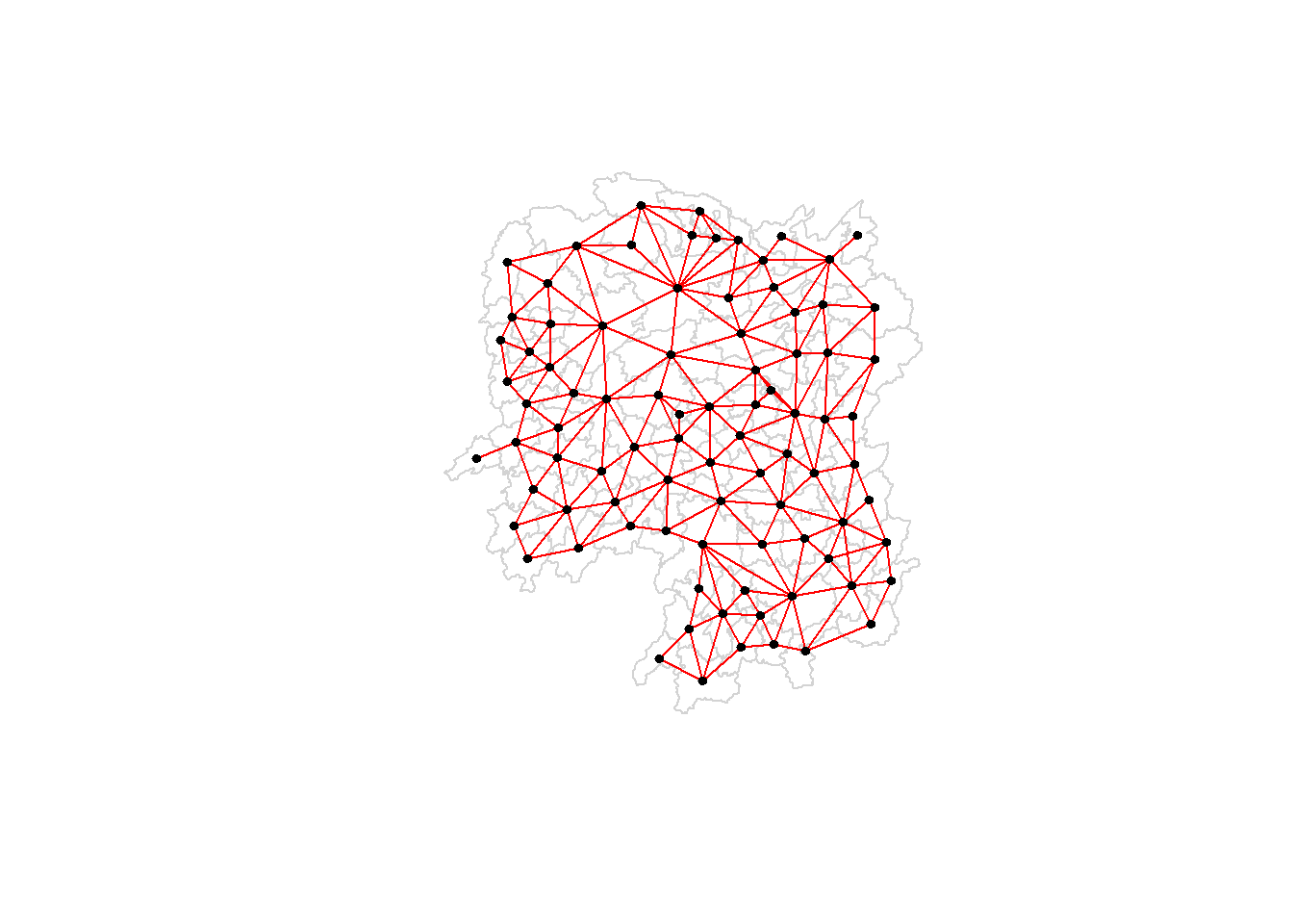
3.3.2 Plotting Rook contiguity based neighbours map
plot(hunan$geometry, border="lightgrey")
plot(wm_r, coords, pch = 19, cex = 0.6, add = TRUE, col = "red")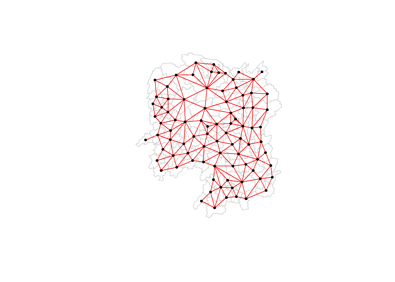
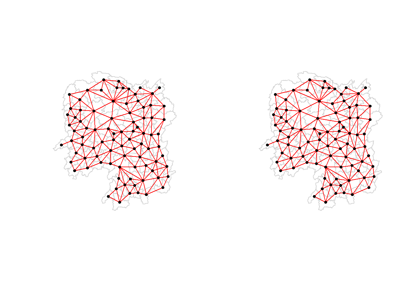
3.3.4 Plotting both Queen and Rook contiguity based neighbours maps
par(mfrow=c(1,2))
plot(hunan$geometry, border="lightgrey")
plot(wm_q, coords, pch = 19, cex = 0.6, add = TRUE, col= "red", main="Queen Contiguity")
plot(hunan$geometry, border="lightgrey")
plot(wm_r, coords, pch = 19, cex = 0.6, add = TRUE, col = "red", main="Rook Contiguity")