In-class Exercise 2: Geospatial Data Wrangling

Author

Tiffanik

Published

January 20, 2023

Modified

March 27, 2023

Getting Started

Installing and loading R packages

In this section, I will install and load tidyverse and sf packages.

pacman::p_load(sf, tidyverse, funModeling)

The geoBoundaries data set

geoNGA <- st_read("data/geospatial/",
                  layer = "geoBoundaries-NGA-ADM2") %>%
  st_transform(crs = 26392)

Reading layer `geoBoundaries-NGA-ADM2' from data source 
  `C:\tiffanik\IS415-GAA\In-class_Ex\In-class_Ex02\data\geospatial' 
  using driver `ESRI Shapefile'
Simple feature collection with 774 features and 5 fields
Geometry type: MULTIPOLYGON
Dimension:     XY
Bounding box:  xmin: 2.668534 ymin: 4.273007 xmax: 14.67882 ymax: 13.89442
Geodetic CRS:  WGS 84

The NGA data set

NGA <- st_read("data/geospatial/",
               layer = "nga_admbnda_adm2_osgof_20190417") %>%
  st_transform(crs = 26392)

Reading layer `nga_admbnda_adm2_osgof_20190417' from data source 
  `C:\tiffanik\IS415-GAA\In-class_Ex\In-class_Ex02\data\geospatial' 
  using driver `ESRI Shapefile'
Simple feature collection with 774 features and 16 fields
Geometry type: MULTIPOLYGON
Dimension:     XY
Bounding box:  xmin: 2.668534 ymin: 4.273007 xmax: 14.67882 ymax: 13.89442
Geodetic CRS:  WGS 84

Importing Aspatial data

wp_nga <- read_csv("data/aspatial/WPdx.csv") %>%
  filter(`#clean_country_name` == "Nigeria")

Warning: One or more parsing issues, call `problems()` on your data frame for details,
e.g.:
  dat <- vroom(...)
  problems(dat)

Rows: 426774 Columns: 74
── Column specification ────────────────────────────────────────────────────────
Delimiter: ","
chr (46): #source, #report_date, #status_id, #water_source_clean, #water_sou...
dbl (23): row_id, #lat_deg, #lon_deg, #install_year, #fecal_coliform_value, ...
lgl  (5): #rehab_year, #rehabilitator, is_urban, latest_record, is_duplicate

ℹ Use `spec()` to retrieve the full column specification for this data.
ℹ Specify the column types or set `show_col_types = FALSE` to quiet this message.

Write the extracted data into rds format

Converting Aspatial Data into Geospatial

wp_nga$Geometry = st_as_sfc(wp_nga$`New Georeferenced Column`)
wp_nga

# A tibble: 97,478 × 75
   row_id `#source`      #lat_…¹ #lon_…² #repo…³ #stat…⁴ #wate…⁵ #wate…⁶ #wate…⁷
    <dbl> <chr>            <dbl>   <dbl> <chr>   <chr>   <chr>   <chr>   <chr>  
 1 158721 Federal Minis…    5.07    6.62 02/19/… Yes     Boreho… Well    Mechan…
 2 158892 Federal Minis…    5.09    7.09 02/06/… Yes     Boreho… Well    Hand P…
 3 323117 Federal Minis…    5.91    8.77 08/31/… Yes     Boreho… Well    Hand P…
 4 300176 Federal Minis…    5.23    7.32 05/17/… Yes     Boreho… Well    Mechan…
 5 324346 Federal Minis…    6.88    3.36 08/17/… Yes     Boreho… Well    Mechan…
 6 297273 Federal Minis…    6.59    3.29 05/26/… Yes     Boreho… Well    Mechan…
 7 296853 Federal Minis…    6.60    3.26 06/02/… Yes     Boreho… Well    Mechan…
 8 323866 Federal Minis…    6.20    6.73 09/18/… Yes     Boreho… Well    Mechan…
 9 297044 Federal Minis…    6.61    3.30 05/26/… Yes     Boreho… Well    Mechan…
10 324321 Federal Minis…    6.96    3.60 08/16/… Yes     Boreho… Well    Mechan…
# … with 97,468 more rows, 66 more variables: `#water_tech_category` <chr>,
#   `#facility_type` <chr>, `#clean_country_name` <chr>, `#clean_adm1` <chr>,
#   `#clean_adm2` <chr>, `#clean_adm3` <chr>, `#clean_adm4` <chr>,
#   `#install_year` <dbl>, `#installer` <chr>, `#rehab_year` <lgl>,
#   `#rehabilitator` <lgl>, `#management_clean` <chr>, `#status_clean` <chr>,
#   `#pay` <chr>, `#fecal_coliform_presence` <chr>,
#   `#fecal_coliform_value` <dbl>, `#subjective_quality` <chr>, …

wp_sf <- st_sf(wp_nga, crs=4326)
wp_sf

Simple feature collection with 97478 features and 74 fields
Geometry type: POINT
Dimension:     XY
Bounding box:  xmin: 2.707441 ymin: 4.301812 xmax: 14.21828 ymax: 13.86568
Geodetic CRS:  WGS 84
# A tibble: 97,478 × 75
   row_id `#source`      #lat_…¹ #lon_…² #repo…³ #stat…⁴ #wate…⁵ #wate…⁶ #wate…⁷
 *  <dbl> <chr>            <dbl>   <dbl> <chr>   <chr>   <chr>   <chr>   <chr>  
 1 158721 Federal Minis…    5.07    6.62 02/19/… Yes     Boreho… Well    Mechan…
 2 158892 Federal Minis…    5.09    7.09 02/06/… Yes     Boreho… Well    Hand P…
 3 323117 Federal Minis…    5.91    8.77 08/31/… Yes     Boreho… Well    Hand P…
 4 300176 Federal Minis…    5.23    7.32 05/17/… Yes     Boreho… Well    Mechan…
 5 324346 Federal Minis…    6.88    3.36 08/17/… Yes     Boreho… Well    Mechan…
 6 297273 Federal Minis…    6.59    3.29 05/26/… Yes     Boreho… Well    Mechan…
 7 296853 Federal Minis…    6.60    3.26 06/02/… Yes     Boreho… Well    Mechan…
 8 323866 Federal Minis…    6.20    6.73 09/18/… Yes     Boreho… Well    Mechan…
 9 297044 Federal Minis…    6.61    3.30 05/26/… Yes     Boreho… Well    Mechan…
10 324321 Federal Minis…    6.96    3.60 08/16/… Yes     Boreho… Well    Mechan…
# … with 97,468 more rows, 66 more variables: `#water_tech_category` <chr>,
#   `#facility_type` <chr>, `#clean_country_name` <chr>, `#clean_adm1` <chr>,
#   `#clean_adm2` <chr>, `#clean_adm3` <chr>, `#clean_adm4` <chr>,
#   `#install_year` <dbl>, `#installer` <chr>, `#rehab_year` <lgl>,
#   `#rehabilitator` <lgl>, `#management_clean` <chr>, `#status_clean` <chr>,
#   `#pay` <chr>, `#fecal_coliform_presence` <chr>,
#   `#fecal_coliform_value` <dbl>, `#subjective_quality` <chr>, …

wp_sf <- wp_sf %>%
  st_transform(crs = 26392)

Geospatial Data Cleaning

Excluding redundent fields

NGA <- NGA %>%
  select(c(3:4, 8:9))

Checking for duplicate name

NGA$ADM2_EN[duplicated(NGA$ADM2_EN)==TRUE]

[1] "Bassa"    "Ifelodun" "Irepodun" "Nasarawa" "Obi"      "Surulere"

NGA$ADM2_EN[94] <- "Bassa, Kogi"
NGA$ADM2_EN[95] <- "Bassa, Plateau"
NGA$ADM2_EN[304] <- "Ifelodun, Kwara"
NGA$ADM2_EN[305] <- "Ifelodun, Osun"
NGA$ADM2_EN[355] <- "Irepodun, Kwara"
NGA$ADM2_EN[356] <- "Irepodun, Osun"
NGA$ADM2_EN[519] <- "Nasarawa, Kano"
NGA$ADM2_EN[520] <- "Nasarawa, Nasarawa"
NGA$ADM2_EN[546] <- "Obi, Benue"
NGA$ADM2_EN[547] <- "Obi, Nasarawa"
NGA$ADM2_EN[693] <- "Surulere, Lagos"
NGA$ADM2_EN[694] <- "Surulere, Oyo"

NGA$ADM2_EN[duplicated(NGA$ADM2_EN)==TRUE]

character(0)

Data Wrangling for Water Point Data

freq(data = wp_sf,
     input = '#status_clean')

Warning: The `<scale>` argument of `guides()` cannot be `FALSE`. Use "none" instead as
of ggplot2 3.3.4.
ℹ The deprecated feature was likely used in the funModeling package.
  Please report the issue at <https://github.com/pablo14/funModeling/issues>.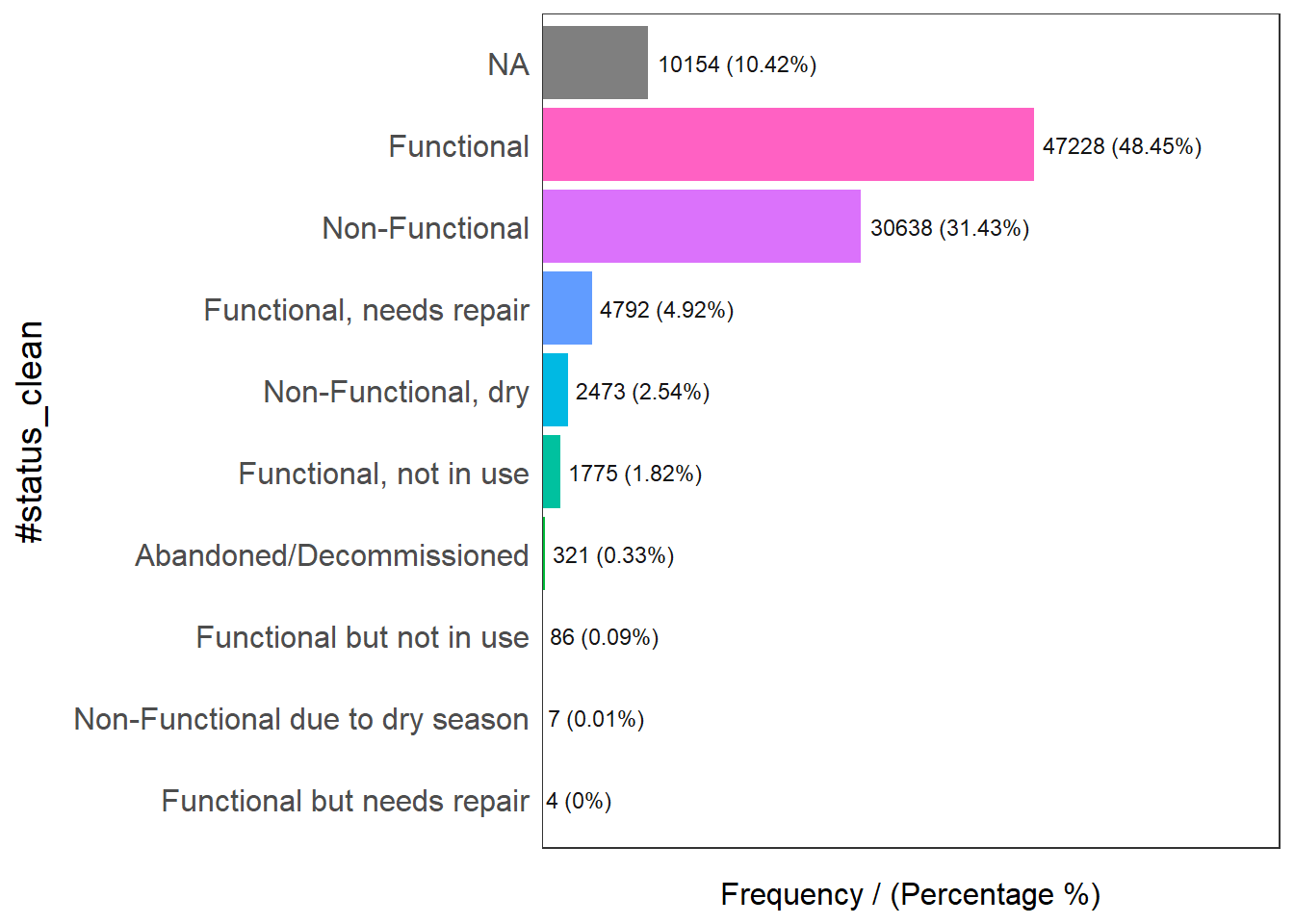

                      #status_clean frequency percentage cumulative_perc
1                        Functional     47228      48.45           48.45
2                    Non-Functional     30638      31.43           79.88
3                              <NA>     10154      10.42           90.30
4          Functional, needs repair      4792       4.92           95.22
5               Non-Functional, dry      2473       2.54           97.76
6            Functional, not in use      1775       1.82           99.58
7          Abandoned/Decommissioned       321       0.33           99.91
8         Functional but not in use        86       0.09          100.00
9  Non-Functional due to dry season         7       0.01          100.01
10      Functional but needs repair         4       0.00          100.00

wp_sf_nga <- wp_sf %>% 
  rename(status_clean = '#status_clean') %>%
  select(status_clean) %>%
  mutate(status_clean = replace_na(
    status_clean, "unknown"))

Extracting Water Point Data

wp_functional <- wp_sf_nga %>%
  filter(status_clean %in%
           c("Functional",
             "Functional but not in use",
             "Functional but needs repair"))

wp_nonfunctional <- wp_sf_nga %>%
  filter(status_clean %in%
           c("Abandoned/Decommissioned",
             "Abandoned",
             "Non-Functional due to dry season",
             "Non-Functional",
             "Non functional due to dry season"))

wp_unknown <- wp_sf_nga %>%
  filter(status_clean == "unknown")

freq(data = wp_functional,
     input = 'status_clean')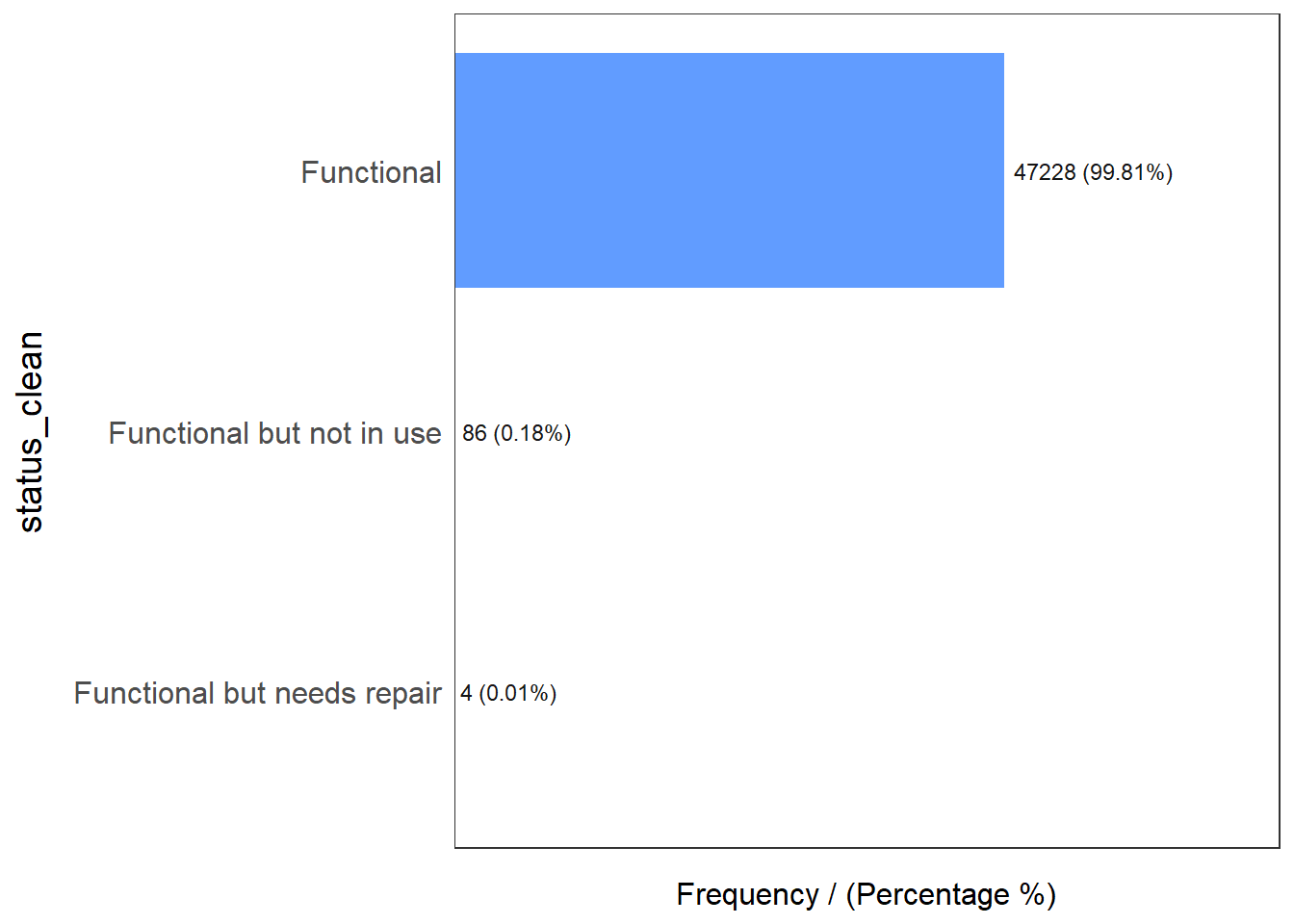

                 status_clean frequency percentage cumulative_perc
1                  Functional     47228      99.81           99.81
2   Functional but not in use        86       0.18           99.99
3 Functional but needs repair         4       0.01          100.00

freq(data = wp_nonfunctional,
     input = 'status_clean')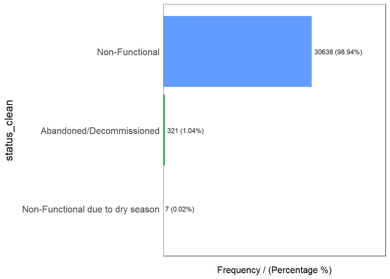

                      status_clean frequency percentage cumulative_perc
1                   Non-Functional     30638      98.94           98.94
2         Abandoned/Decommissioned       321       1.04           99.98
3 Non-Functional due to dry season         7       0.02          100.00

freq(data = wp_unknown,
     input = 'status_clean')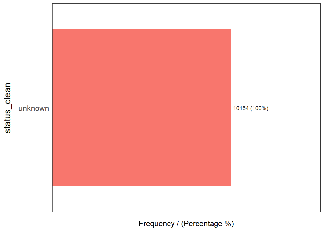

  status_clean frequency percentage cumulative_perc
1      unknown     10154        100             100

Performing Point-in-Polygon Count

NGA_wp <- NGA %>% 
  mutate(`total_wp` = lengths(
    st_intersects(NGA, wp_sf_nga))) %>%
  mutate(`wp_functional` = lengths(
    st_intersects(NGA, wp_functional))) %>%
  mutate(`wp_nonfunctional` = lengths(
    st_intersects(NGA, wp_nonfunctional))) %>%
  mutate(`wp_unknown` = lengths(
    st_intersects(NGA, wp_unknown)))

Visualing attributes by using statistical graphs

ggplot(data = NGA_wp,
       aes(x = total_wp)) + 
  geom_histogram(bins=20,
                 color="black",
                 fill="light blue") +
  geom_vline(aes(xintercept=mean(
    total_wp, na.rm=T)),
             color="red", 
             linetype="dashed", 
             size=0.8) +
  ggtitle("Distribution of total water points by LGA") +
  xlab("No. of water points") +
  ylab("No. of\nLGAs") +
  theme(axis.title.y=element_text(angle = 0))

Warning: Using `size` aesthetic for lines was deprecated in ggplot2 3.4.0.
ℹ Please use `linewidth` instead.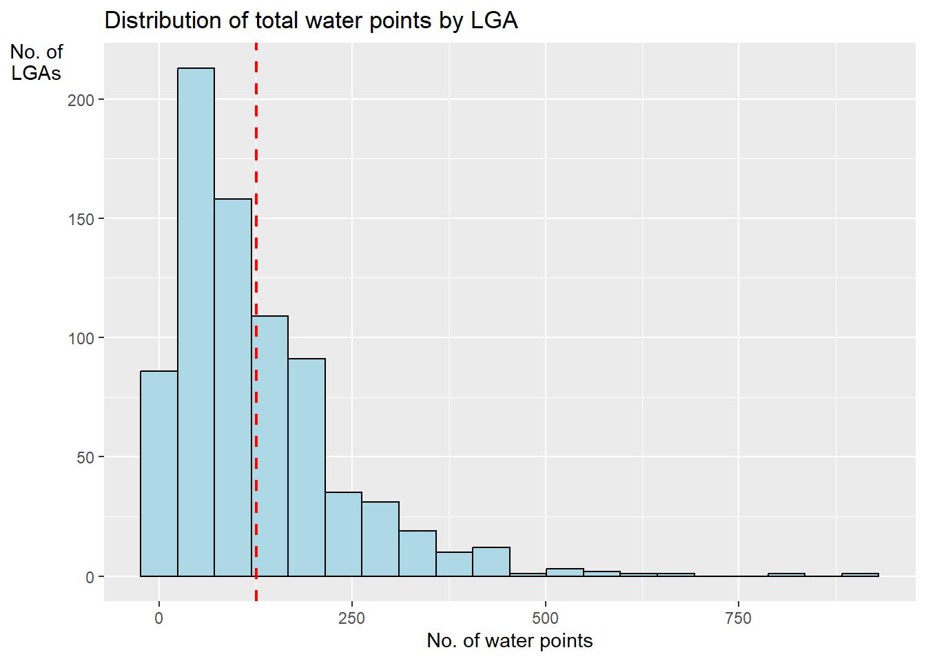

Saving the analytical data in rds format

write_rds(NGA_wp, "data/rds/NGA_wp.rds")